A Star is Born
By Sophia Kressy
Regardless of whether you prefer Barbara Streisand’s or Lady Gaga’s version, how a star is born is an exciting question. In this case, we mean a fiery ball of burning gas, not a dazzling primadonna.
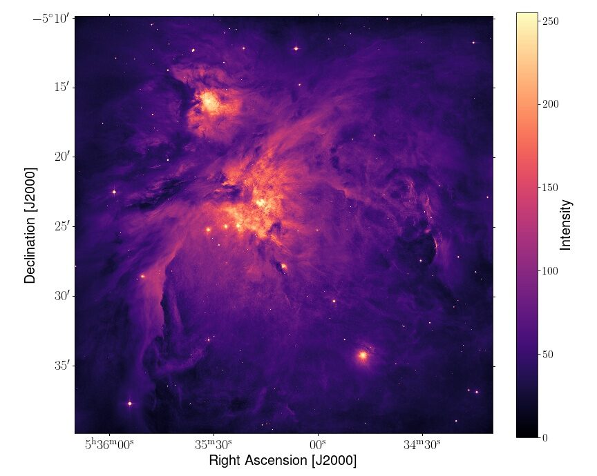
Stars form in the densest regions of interstellar molecular clouds, namely in filaments or dense cores. Filaments are long, finger-like striations of dense gas that form as a cloud gravitationally collapses. Material in these filaments collapse further into even denser cores. Within cores, star formation begins. The Orion Molecular Cloud (OMC), shown in Figure 1, is an example of a star forming region.
Gravity, turbulence, stellar feedback and magnetic fields are the primary ingredients for star formation. Gravity is the main driver. It dominates the collapse and eventual birth of the star. Turbulence and stellar feedback churn and mix the gas and material. Stellar feedback is caused by stars releasing massive amounts of energy, namely in the form of stellar winds, protostellar jets, and supernovae. Turbulence and stellar feedback sometimes help or hinder star formation, depending on the scale we look at. Magnetic fields, however, may provide support against gravitational collapse, potentially slowing down star formation.
Although theories predict about 300 stars to form every year in our Milky Way galaxy, only about 1 star is born every year. One explanation for this discrepancy is magnetic fields. Magnetic fields can become tied to the gas through a process known as “flux-freezing.” They can create pressure and tension in the cloud through this process and potentially slow the collapse.
The Flat Stanley Predicament
Magnetic fields are elusive to astronomers in that our measurements of them are constrained.
Dust grains in an interstellar molecular cloud can become partially aligned to the clouds magnetic field. The dust grains absorb background starlight and re-radiate it, imparting a polarization signature onto the emitted light. Astronomers observe this polarized light and can discern the orientation of the magnetic field in the plane-of-sky.
Astronomers have ways of inferring the line-of-sight magnetic field, but no method of directly observing it. This means that there is a missing dimension in magnetic field measurements, namely that the three-dimension structure of magnetic fields cannot be observed directly.
And so, similar to the iconic storybook character, magnetic fields will forever remain in two-dimensions, like Flat Stanley.
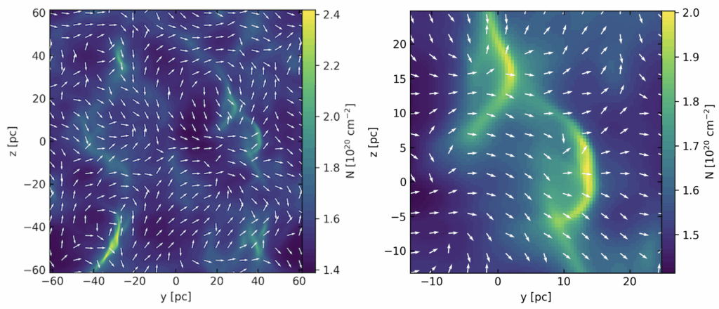
The goal of this research project is to reconstruct the 3D magnetic field structure. By using data available on the magnetic field (polarization maps; see Fig. 2) and the cloud (density, temperature, velocity), we can reconstruct the 3D magnetic field with statistical analysis.
A Method for 3D Magnetic Fields
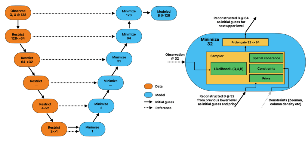
Figure 3 summarizes the structure of the reconstruction procedure. Information from dust-polarization maps, in orange, enters at the top left at a given resolution (here 1282 points).
Following the solid arrows, the observed data are “restricted” by a factor of 2 from (map128) down to (map1), leaving us with the “observation” in one cell. “Restriction” essentially averages the observed data into coarser resolution maps, which can provide different initial starting points for the reconstruction. This prevents the software from being bias towards its initial starting point.
Moving to the bottom of the blue branch, the one cell (map1) is “reconstructed” to the full 3D field orientation. We can initially reconstruct the 3D field with equations derived from polarimetry (the study of polarized light), but we need to sample these results to explore options and produce a statistically significant value. A Metropolis-Hastings Markov Chain was used for this sampler, sketched out on the right of Fig. 3. This sampler allows us to test a large parameter space, which translates to essentially trying on various “hats” and seeing what best “fits” our initial conditions. We can also add additional information (spatial coherence, constraints, and priors) to make our hat “fit” better.
We find the most probable reconstructed values (i.e. calculate likelihood) from the sampled values, and those are accepted. The single-cell reconstruction is then interpolated to the next higher level (“2”) and used as initial guess and prior for the next sampling step. This process is iterative until the highest level, or resolution (1282), is met.
The result is the most probable 3D magnetic field components, which produces the sought-after reconstructed, or modeled, 3D magnetic field (Fig. 3; blue, top-right).
Moving Forward
The reconstruction method has been tested with idealized magnetic field geometries (uniform, wavy, hourglass), with no cloud or dust grain information. In the future, testing with magnetohydrodynamical simulations with full physics will be implemented to calibrate the software further. The result will be a software that can take 2D dust-polarization maps from observed star forming regions and return a reconstructed 3D magnetic field morphology. The reconstruction software will be publicly available to the astrophysics community, in the hopes of unraveling how magnetic field structure effects how a star is born.
Sophia Kressy is a Ph.D. candidate in astrophysics at the University of North Carolina. She is a North Carolina Space Grant Graduate Research Fellow.